Here is an example of MATLAB code that was developed for 1D conduction heat transfer problems. This code was developed for MECH 302 – Finite Element Analysis at Bucknell. Specifics of this code include the following:
- User inputs for:
- Geometry, conduction coefficient, and mesh density
- Distributed internal heat generation as a function of location
- Essential, natural, and mixed boundary conditions
- Quadratic 1D elements
- A Gaussian Quadrature MATLAB function
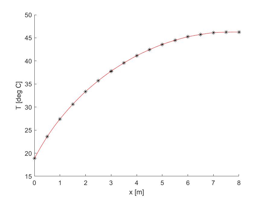
- A plot of temperature and the derivative of temperature as a function of location
- The value of the maximum nodal temperature
- The temperature value of a specific location as specified by the user
- Boundary heat flux
The code is not published online because it’s an assignment for the course, but please feel free to email me (b.wheatley@bucknell.edu) and I would be happy to share.
Here is an example of the code at work:

Input domain length in [m]: 8
Input number of elements: 8
Input conduction coefficient k in [W/m-C]: 200
Input initial area [m^2]: 0.1
Input final area [m^2]: 0.5
Input distributed internal heat generation [W/m^3] as a function of x: 10*x
Specify boundary conditions as follows: 1 - known temperature, 2 - known flux, 3 - convection.
Specify left boundary condition type: 3
Specify left convection coefficient in [W/m^2-C]: 50
Specify left fluid temperature in [deg C]: 10
Specify right boundary condition type: 2
Specify right flux in [W]: 0
The maximum temperature is 46.26 [deg C].
The maximum temperature location is 8 [m].
Specify location of desired approximation in [m]: 7.5
The temperature at x = 7.5 [m] is 46.13 [deg C].
Heat flux at left boundary is -210.4 [W].
Heat flux at right boundary is 0 [W].